Data Quality Metrics Examples: The Complete Guide

Data quality metrics are the quantifiable measures (e.g,, percent of NULL values in a column) used to assess the integrity, validity, and reliability of data within an operational pipeline. Unlike quality dimensions, which are more abstract in nature (e.g., “accuracy”), metrics represent the specific, computable logic used to enforce those dimensions.

This article illustrates examples of four categories of data quality metrics that together allow assessment of the eight key dimensions of data quality:

• Accuracy: Data correctly reflects real-world entities.
• Completeness: All necessary data is present, with no missing values in mandatory fields.
• Consistency: Data is uniform and does not conflict across different systems or datasets, and is stable over time.
• Volumetrics: Data volume follows expected patterns.
• Timeliness (Freshness): Data is available when needed and up-to-date.
• Conformity: Data matches defined formats and types.
• Precision: Field granularity and values meet range and temporal boundary constraints.
• Coverage: A meta-metric checking that all fields have sufficient active quality checks.

{{banner-large-1="/banners"}}

Key categories of data quality metrics examples

This article covers examples of data quality metrics in the following categories.

The role of data quality metrics

Data quality metrics have three main purposes:

• Detection: Identifying defects in data before they propagate downstream (e.g., making sure that a daily ingestion file is not be empty)
• Standardization: Translating abstract quality dimensions (accuracy, completeness, timeliness, etc.) into computable checks (e.g., checking that customers_interested entries have an email address)
• Control: Providing thresholds that can trigger alerts, block pipelines, or initiate remediation workflows (e.g., if today's invoice staging table contains zero records then halt accounting sync and alert stakeholders)

In modern data reliability engineering, these metrics act as the service-level indicators (SLIs) for data. SLIs are metrics that measure the performance and reliability of a service from a user's perspective. They function across three distinct architectural layers:

1. Deterministic validation: Boolean checks against known constraints (e.g., NOT NULL, RegEx match)
2. Probabilistic monitoring: Statistical analysis of data distributions to detect anomalies without static thresholds (e.g., deviation from mean)
3. Operational metadata: Analysis of pipeline telemetry (latency, volume) rather than cell values

Designing effective data quality metrics

Useful metrics have the following qualities:

• Transparency: The metric can be traced back to the exact records responsible for the score. Transparency ensures that quality metrics are debuggable, not just observable.
• Context: Weighting logic that assigns higher criticality to fields influencing downstream consumption. Some values are more important than others, and their context matters. A missing middle initial does not carry the same weight as a missing surname, and a missing surname may be ok if the customer is an organization.
• Actionability: The metric must trigger a specific remediation workflow or alert routing. Metrics are actionable if they trigger a clear response when thresholds are exceeded. Values in daily reports may be useful in some contexts but may lead to delayed detection or entirely missing critical issues.
• Adaptiveness: The ability of the metric baseline to evolve via machine learning as data distributions shift. As time passes, volumes increase and usage patterns shift. Thresholds based on fixed values (e.g. a daily ingestion file that must process in under 60 minutes) may start triggering frequent alerts due to business growth over time. Ratios, especially ratios based on period over period (PoP), as well as mean and average values, can help maintain the validity of a metric or threshold over time.

Each metric operates at a specific granularity level: field (column), container (table), or datastore (system). This determines both the scope of what it measures and how its results are aggregated into higher-level quality scores.

Achieving these qualities manually would involve writing SQL that drills to record level and records every instance that triggers a metric, configuring weighted alerting, and building and maintaining adaptive thresholds. The engineering effort and ongoing maintenance required by this would quickly become impossible for anything more than very small data stores. You need a data quality platform like Qualytics that can automate this by connecting directly to your data sources, inferring ~95% of the necessary checks automatically, surfacing the specific records behind every metric score, routing alerts to the right owners, and learning and adjusting baseline distributions over time so thresholds stay valid as your data evolves.

Fundamental integrity metrics

Fundamental integrity metrics ensure that data is structurally valid (i.e., not broken) at the system level, validating properties like whether required fields are present, keys are valid and consistent, or constraints are respected. A dataset with missing keys, invalid references, or unresolvable foreign keys cannot be reliably processed or analyzed.

These metrics are typically enforced at the ingestion and transformation stages, where they act as the first line of defense against poor-quality data entering the system. Fundamental integrity checks contribute primarily to assessing the completeness dimension of data quality. The coverage meta-metric is often also considered a fundamental integrity metric.

The following specific examples illustrate the concepts and show the usefulness of these metrics.

Null rate (field-level completeness)

This metric is the ratio of records in which a given field contains a null (missing) value relative to the total number of records that should have a value. 

In a traditional data quality setup, a data engineer might write the following SQL code to compute this metric for a single field:

SELECT CAST(COUNT(*) FILTER (WHERE date IS NULL) AS double precision) / COUNT(*) AS orders_with_null_date
FROM orders

‍

Note that this example lacks transparency and context as defined above. Because the query returns only an aggregate ratio, there is no way to trace the score back to the specific records containing null values, making it observable but not debuggable. It may be actionable in terms of triggering an alert at a pre-defined threshold, but it will be harder to track down and remedy since the offending fields are not identified. Modern data quality platforms address this issue by surfacing the specific records responsible for a metric’s value, enabling engineers to move directly from detection to remediation. 

The example rule also does not provide any information about how critical a null order date is. A platform like Qualytics allows you to add prioritization and categorization tags to any datastore, field, check, etc., helping you appropriately prioritize your anomaly response.

In a manual system, a rule like this would be associated with a fixed threshold. In a modern data quality platform, an initial threshold can be set automatically based on data profiles, and this can adapt over time based on observed data patterns and engineer feedback, reducing alert fatigue as the system learns what's normal. 

The SQL examples throughout this article illustrate how each metric might be computed, but most will share the same limitations: They produce aggregate scores without record-level traceability, lack context-aware or adaptive thresholds, and require manual wiring to alerting or remediation workflows.

Record completeness (container-level completeness)

This metric is the percentage of records satisfying a “minimal viable record” definition (all mandatory keys present, such as primary keys and foreign keys). Here’s example code for this metric:

SELECT CAST(COUNT(*) FILTER (
    WHERE date IS NOT NULL
      AND client_id IS NOT NULL
      AND quote_amount IS NOT NULL
    ) AS double precision) / COUNT(*) AS orders_completion_rate
FROM orders

Orphan rate (container-level completeness)

As an example, if a record is deleted from the customer table but associated orders still remain in the orders table, those orders are orphaned. The customer_id still looks valid, but it no longer exists in the customer table, so the order is now invalid. 

In systems that enforce referential integrity at ingestion (rejecting orders with nonexistent customer IDs), the only way this situation occurs is via deletion of customer records that are still needed. However, many modern data architectures, including data lakes and event-driven pipelines, do not enforce referential integrity at ingestion, so orphaned records can also result from incomplete or out-of-order data arrival. This metric catches such integrity violations.

This SQL code computes the orphan rate as the percentage of records in the billing.orders table that have a customer_id not found in crm.customers.

SELECT CAST(COUNT(*) FILTER (
    WHERE customer_id NOT IN (
        SELECT id FROM crm.customers
        )
    ) AS double precision) / COUNT(*) AS order_orphan_rate
FROM billing.orders

Monitoring density (field- or container-level coverage)

This meta-metric measures how well the data is being checked rather than how good it is, and it can identify data catalogs where governance should be in place but is absent. 

For example, as part of monitoring density, one can calculate the table-level density and column-level coverage in the following way: 

table_level_density = total_checks / total_tables

column_level_coverage = columns_with_checks / total_columns

A weighted coverage metric can assign different weights to each table or column according to how critical that data is. You can also weight by check diversity, which measures how many of the core dimensions are covered for a given field. Strong coverage requires a mix of different types of checks (i.e., not just “null” but also freshness, accuracy, distribution, etc.).

This can look something like:

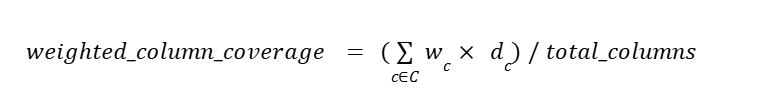
Where:

C is the set of columns with checks;

w_с is the importance weight of column c; and

d_c is the diversity of the checks in place for column c (e.g., dimensions_covered / 8

Form and structure metrics

These metrics ensure that data is usable, interpretable, and consistently represented. They validate how data is formatted, encoded, and structured across datasets. Unlike fundamental integrity metrics, which focus on whether data is broken, form and structure metrics focus on whether data can be reliably processed.

This category includes conformity metrics that measure how well data complies with predefined rules, definitions and constraints, such as the following.

Phone number structure (field-level conformity)

The regex rule below requires phone numbers to conform strictly to a (404) 555-1212 format. The rule computes the proportion of conforming values within the field.

SELECT CAST(COUNT(*) FILTER (
    WHERE phone ~ '^\([0-9]{3}\) [0-9]{3}-[0-9]{4}$'
    ) AS double precision) / COUNT(*) AS phone_format_conformity_rate
FROM crm.customers

Type correctness (field-level conformity)

In the case of data architectures where structured data is stored as JSON objects rather than discrete typed columns—such as when the schema is flexible or when documents are ingested wholesale from an API or event stream—it’s possible to ingest data where some field contents are improperly typed. A common pitfall is numbers being represented as strings. 

In this example, invoice lines are stored as a JSONB array (a binary database representation of JSON data) within an invoice record rather than as structured rows in an invoice_lines table. The database schema enforces only that the column must contain well-structured JSON; it has no say regarding the types of values within the JSON structure. Thus, if an invoice line contains an element {"amount": "105.20"}, in many cases this would go unnoticed, but such a value is likely to break downstream processing that requires a numeric value. 

This type of error can be detected with the following code:

SELECT COUNT(*) AS invoices_with_invalid_line_amount_type
FROM billing.invoices i
WHERE i.lines @? '$[*].amount.type() ? (@ <> "number")'

Schema conformity (datastore-level conformity)

Within a traditional SQL or other strongly-typed database, you don’t need a check for table-level conformity because the database takes care of that for you. However, for verifying conformity across two systems (for example, staging versus production), you could use a check such as this one:

SELECT expected.column_name
FROM information_schema.columns expected
WHERE expected.table_name = 'new_customers'
AND expected.table_schema = 'staging'
AND NOT EXISTS (
    SELECT 1 FROM information_schema.columns actual
    WHERE actual.table_name = 'customers'
    AND actual.table_schema = 'crm'
    AND actual.column_name = expected.column_name
    AND actual.data_type = expected.data_type
)

‍

Note that in modern data platforms like Snowflake or BigQuery, schema enforcement is more permissive, and in data lakes, the schema is inferred or defined at read time (schema-on-read). In these environments, schema drift can occur silently, and conformity checks require platform-native tooling or a dedicated data quality layer, going beyond what SQL-based checks can provide. 

Price precision compliance (field-level precision)

The form and structure category also includes numeric resolution/precision metrics. Resolution refers to the smallest measurable increment a value can have, and precision is the number of significant digits or decimal places. For example:

SELECT CAST(COUNT(*) FILTER (
    WHERE SCALE(unit_price) = 2
    ) AS double precision) / COUNT(*) AS unit_price_precision_compliance_rate
FROM billing.invoice_lines

‍

This metric assesses the proportion of unit_price entries that have the required two decimal places of precision expected for monetary values. This level of precision sets the price resolution to one cent ($0.01). Note: This example uses PostgreSQL’s SCALE() function, which returns the number of decimal places in a numeric value. Equivalent functionality varies by SQL dialect.

Value and consistency metrics

These metrics verify that the data correctly represents the real world (accuracy) and remains uniform and consistent over time across systems (consistency), focusing on semantic correctness and cross-system alignment.

Cross-field relationships (field-level accuracy)

One example of an accuracy metric would be ensuring that an employee’s hire date is later than their birth date. This SQL code computes the proportion of records for which that is not true:

SELECT CAST(COUNT(*) FILTER (
    WHERE hire_date < birthdate
    ) AS double precision) / COUNT(*) AS invalid_hire_date_rate
FROM hr.employees

‍

Another example would be ensuring that the relationship between square footage and price of a property remains consistent. Here we have a sample rule that enforces prices between 800 and 1,200 times the square footage. Ideally, this check would not be static—the boundaries would be inferred from patterns identified by profiling the data.

SELECT CAST(COUNT(*) FILTER (
    WHERE price < (square_footage * 800)
    OR price > (square_footage * 1200)
    ) AS double precision) / COUNT(*) AS property_price_accuracy_rate
FROM real_estate.listings

Cross-system consistency (datastore-level consistency)

This metric checks that fields derived from a system of record (SOR) remain consistently aligned with that source of truth. For example, the CRM and billing modules both record a customer’s plan or tier; these should be aligned, but the CRM is the system of record, as CRM is where the sales and account management teams originate and maintain this information. Billing should be consulting and consuming this information. 

This code detects SOR drift, where billing data becomes misaligned with this authoritative source:

SELECT CAST(COUNT(*) FILTER (
    WHERE c.tier <> a.plan
    ) AS double precision) / COUNT(*) AS plan_fidelity_rate
FROM crm.customers c
JOIN billing.accounts a ON (a.customer_id = c.id)

Statistical distribution stability (field-level consistency)

Another important type of consistency check is the extent to which a field's statistical shape and distribution remain stable over time. This example compares the median unit_price between two consecutive weeks and computes the percent change.

SELECT 
    PERCENTILE_CONT(0.5) WITHIN GROUP (ORDER BY unit_price) 
        FILTER (WHERE created_date >= CURRENT_DATE - INTERVAL '7 days') 
        AS current_week_median,
    PERCENTILE_CONT(0.5) WITHIN GROUP (ORDER BY unit_price) 
        FILTER (WHERE created_date BETWEEN CURRENT_DATE - INTERVAL '14 days' 
        AND CURRENT_DATE - INTERVAL '7 days') 
        AS prior_week_median,
    CAST(
        PERCENTILE_CONT(0.5) WITHIN GROUP (ORDER BY unit_price) 
            FILTER (WHERE created_date >= CURRENT_DATE - INTERVAL '7 days') -
        PERCENTILE_CONT(0.5) WITHIN GROUP (ORDER BY unit_price) 
            FILTER (WHERE created_date BETWEEN CURRENT_DATE - INTERVAL '14 days' 
            AND CURRENT_DATE - INTERVAL '7 days')
        AS double precision) /
    NULLIF(PERCENTILE_CONT(0.5) WITHIN GROUP (ORDER BY unit_price) 
        FILTER (WHERE created_date BETWEEN CURRENT_DATE - INTERVAL '14 days' 
        AND CURRENT_DATE - INTERVAL '7 days'), 0) 
        AS median_drift_rate
FROM billing.invoice_lines

‍

For example, if the prior week’s median is $45.00 and the current week’s median is  $4,500.00, this check would compute a median_drift_rate of 9,900%. A threshold, either set manually based on business rules or automatically based on historical data, would then be applied to see whether to raise an alert. This type of rule is important because it would surface a dramatic shift that no conformity or accuracy check would catch, since every individual value may be correctly formatted and within a plausible range.

Operational health metrics

These metrics measure the behavior of the data pipeline rather than the content of the data itself. They track whether data is delivered on time, at the expected volume, and with consistent throughput. Data can be structurally valid and semantically correct and yet still be unusable if it arrives late or incomplete.

Data latency (datastore-level freshness)

One of the most important operational health metrics is data latency, which measures how long it takes for data to become available after it is generated. This metric area highlights the difference between correctness and usefulness. If latency is too high, the data may be technically correct but still be useless for the business or organization. 

Latency can be subdivided as follows:

• Ingestion latency: The time between the creation of the event and the availability of the data in the system
• Processing latency: The time between the start and finish of data processing or transforming processes.
• End-to-end latency: What the business actually feels, e.g., the time from an event to its data being usable in a dashboard or model

‍

Suitable latency thresholds depend on the processes that depend on the data, for example, for real-time systems, seconds may matter; for dashboards, it may be more on the order of minutes; for reporting, hours or days may be okay.

Volumetric deviation (container-level volumetrics)

Another important metric in this category is volumetric deviation, which measures the actual volume of incoming or processed data compared to the expected volume. The expected volume could be defined by historical volumes, current batch size, or other known business characteristics.

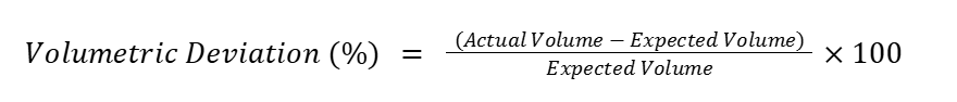
This is very effective for detecting silent failures where, for example, a job completes successfully or without any warnings or errors but extracts zero rows or extracts all duplicates (doubling the number of rows). Those problems would represent volumetric deviations of –100% and +100% respectively.

Best practices when monitoring data quality metrics

Effective data quality monitoring requires integrating metrics into the operational behavior of data systems. The following practices help ensure that metrics produce reliable signals and lead to timely remediation.

Validate at the source

When bad data is ingested, it propagates downstream, becoming harder to trace and more expensive to correct. It impacts analytics and business decisions. To avoid this, it is best to deal with bad data straight at the source, during ingestion, rejecting or quarantining bad records, using a staging area as shown below:

UPDATE staging.new_customers SET
    valid = CASE
       WHEN id IS NULL OR id = '' OR id LIKE '%[^0-9]%' THEN 0
       WHEN CAST(id AS INT) IN (SELECT id FROM crm.customers) THEN 0
       WHEN name IS NULL OR TRIM(name) = '' THEN 0
       WHEN email IS NULL OR email NOT LIKE '%_@_%.%' OR email LIKE '% %' THEN 0
       ELSE 1 END
WHERE import_id = 15;

INSERT INTO crm.customers (id, name, email)
SELECT CAST(id AS int), name, email
FROM staging.new_customers
WHERE import_id = 15 AND valid = 1;

‍

Using staging for imports, all values are accepted into the staging area, but only new customers with a valid id, name, and email are imported into the CRM, with the rest marked as invalid and quarantined for later evaluation and correction. This method prevents invalid customer information from corrupting downstream processes.

Automate anomaly detection

Static rules cannot detect unexpected shifts in data behavior, but automated anomaly detection leverages historical baselines to identify deviations without needing to rely on predefined thresholds. For example, suppose a daily job has produced around 50,000 records for a while, but one day it produces only 12,000. The team might wonder how significant this deviation is. The following code finds the mean and standard deviation of the daily counts over the past 90 days and then allows you to check whether any day’s new invoices count falls further than two standard deviations from the mean. (For datasets with skewed distributions, thresholds based on the median and interquartile range may be more appropriate.)

WITH historical_stats AS (
    SELECT 
        AVG(daily_count) AS mean_count,
        STDDEV(daily_count) AS stddev_count
    FROM (
        SELECT COUNT(*) AS daily_count
        FROM staging.new_invoices
        WHERE date BETWEEN CURRENT_DATE - INTERVAL '91' DAY
        AND CURRENT_DATE - INTERVAL '1' DAY
        GROUP BY date
    ) daily_counts
)
SELECT 
    CAST(
        (SELECT COUNT(*) FROM staging.new_invoices
        WHERE date = CURRENT_DATE - INTERVAL '1' DAY)
        AS double precision) /
    NULLIF(mean_count, 0) AS new_invoices_drift_rate,
    mean_count - (2 * stddev_count) AS lower_threshold,
    mean_count + (2 * stddev_count) AS upper_threshold
FROM historical_stats

‍

Adaptive metrics and thresholds using historical baselines remain relevant even as the business evolves. Qualytics can simplify this kind of check for you by continuously profiling historical distributions so that anomaly thresholds reflect your data’s real distribution rather than human guesses. And if there’s seasonality to your data, Qualytics can take that into account as well. A small number of records during your peak season is more concerning than the same number during the off season. 

Use circuit breakers

Some data quality issues require immediate pipeline termination instead of just generating an alert. For example, seeing no records in the current day’s new invoices staging table should trigger a circuit breaker terminating the accounting sync pipeline.

Using the same example as above, a circuit breaker might use a threshold for values beyond five standard deviations from the mean, interrupting the pipeline altogether on an extremely small or excessively large import while maintaining the above example’s non-blocking monitor to alert for less severe variance. 

Prioritize alerts

A system producing too many alerts without relevant priority creates what is known as alert fatigue, causing engineers to deprioritize and even mute notifications. Prioritizing your alerts into tiers based on criticality ensures that your most critical alerts get the timely attention they deserve. For example:

Track coverage

Coverage metrics measure how much of the data is subject to quality checks. For example, a data dictionary with quality check metrics can be compared regularly with system dictionaries, detecting newly added columns or tables without data quality metrics as follows:

SELECT CAST(COUNT(*) FILTER (
    WHERE cc.checks IS NOT NULL
    ) AS double precision) / COUNT(*) AS data_quality_coverage_rate
FROM information_schema.columns cc
LEFT JOIN data_quality.columns qc ON (qc.table_name = cc.table_name 
    AND qc.column_name = cc.column_name)
WHERE cc.table_schema IN ('crm', 'billing')

‍

If a new CRM table is added without data quality checks, this coverage rate drops, potentially triggering an alert.

Monitoring the percentage of fields actually being checked ensures that high scores aren't hiding unmonitored blind spots. This metric can be extended to cover not just columns but also pipelines and other processes where data quality checks are relevant.

Define service-level objectives (SLOs)

SLOs are measurable internal engineering targets for a service’s performance and reliability. Without clearly defined targets, metrics cannot be used to evaluate system performance or trigger escalation. 

When defining SLOs, ensure that metrics are explicit. For example, define metrics like “99.9% of records must be available within 5 minutes of event time” rather than “data should be fresh.”

In order to establish clear engineering standards, SLOs should:

• Define numeric targets for key metrics
• Align thresholds with business impact
• Monitor compliance over time
• Specify a response protocol when targets are breached

SLOs provide a shared standard against which your data quality metrics can be evaluated. They should also provide a remediation protocol for when they are not met. This can include notifications, triggered workflows, alerts to downstream users, and even temporary pipeline blocks until remediation can be achieved. Without SLOs, individual metrics exist in isolation, and your business lacks a principled picture of what “good” data quality looks like. 

Version control your metric definitions 

Data quality rules evolve as systems change. Without version control, it becomes difficult to track when and why a metric was modified. Treating metrics as code and managing them through Git or another version control system ensures reproducibility, auditability, and controlled change management. However, this requires an intentional and reliable process for rule modifications.

Consider a case where a threshold changes from 1% to 10% without any associated ticket, versioned code change, or documented justification. Later, someone discovering this change may wonder: Who made this change? Why was it necessary? Was it deliberate, or a workaround to suppress an alarm?

Data quality platforms like Qualytics manage rule definitions, thresholds, and alert configurations centrally and handle versioning automatically. This eliminates any gap between documented intent and actual runtime configuration. 

Measure mean time to resolve (MTTR)

Detection alone does not improve data quality. The effectiveness of a monitoring system depends on how quickly issues are resolved. MTTR measures the time between detection (metric breach) and resolution (data corrected or pipeline fixed).

For example, consider an outage in a service provider relied on by two companies. Both companies detect the outage at the same time, but company A resolves the problem in 15 minutes, whereas company B resolves it in 6 hours. Both have detection, but only one has effective operations.

Track MTTR for data quality incidents, identifying bottlenecks in investigation and remediation. Use MTTR as a feedback loop to improve alerting and processes.

{{banner-small-1="/banners"}}

Last thoughts

Data quality does not improve through isolated checks or dashboards but rather when metrics are treated as part of the system’s operational control surface. This requires moving from ad hoc validation to structured measurement, i.e.:

• From dimensions to computable metrics
• From passive monitoring to enforced thresholds
• From detection to controlled remediation

Organizing metrics across integrity, structure, value/consistency, and operational health lets engineering teams build a layered approach to data reliability. In practice, the effectiveness of these metrics depends less on their definition and more on how they are implemented, i.e., whether they are actionable, are traceable, and evolve with the system.

While a well-designed data quality framework such as the one Qualytics offers cannot eliminate all defects, what it can do is ensure that defects are detected early, understood quickly, and resolved consistently.